Our client is a hospitality technology company that sees bookings at connected properties as they happen. We run two forecasting systems on that data:
- Property demand forecasting (PDF) predicts room-night occupancy for an individual hotel, from 1 to 90 days ahead of a stay date. Hoteliers use it to decide what to charge and when.
- Market demand forecasting (MDF) predicts aggregate demand for a geographic cluster of hotels, then shares it out to each property in the cluster.
Both ran in production for a few launch countries, chosen because they had the deepest booking history. The ask was to cover more than 50.
MDF scaled in about two weeks with its core pipeline unchanged. PDF took more than a month: the moment we switched it on across the new countries, accuracy fell off a cliff.
What follows is how we got it back. The short version: we barely touched the model. Almost all of the recovery came from feature engineering, backed by a change to how we measured ourselves and one defensive data-quality fix.
The setup
Mechanically, PDF isn’t time-series extrapolation. It’s supervised regression: for a given hotel, stay date and forecast horizon, predict the room nights that will eventually be booked. One gradient-boosted model serves every hotel in a regional group, trained per band of horizons, so a hotel with little history of its own still benefits from patterns learned across the rest of its group.
Both systems follow the same six-stage MLOps pattern on Databricks:
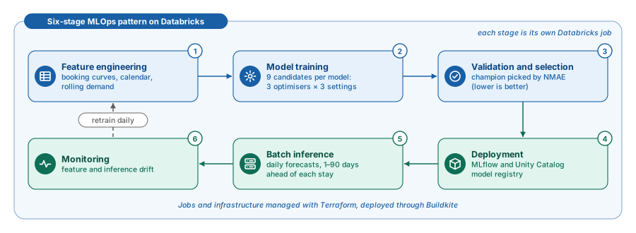
Each stage is its own Databricks job. Training fits nine candidates per model (three optimisers × three hyperparameter settings) and picks a champion by normalised mean absolute error (NMAE). Models live in MLflow and Unity Catalog; jobs and infrastructure are managed with Terraform and deployed through Buildkite.
The target architecture: one model became 75
The single launch-country model became a matrix:
- 5 regional country groups: South-East Asia, Oceania, the Americas, Europe, and the Middle East and Africa
- 15 horizon bands: from 1 day, 2 days and 3 days, up through 81–90 days
That’s 75 small, independent training tasks per system per daily run. Each one finishes well within job time limits and can be retried or rerun on its own.
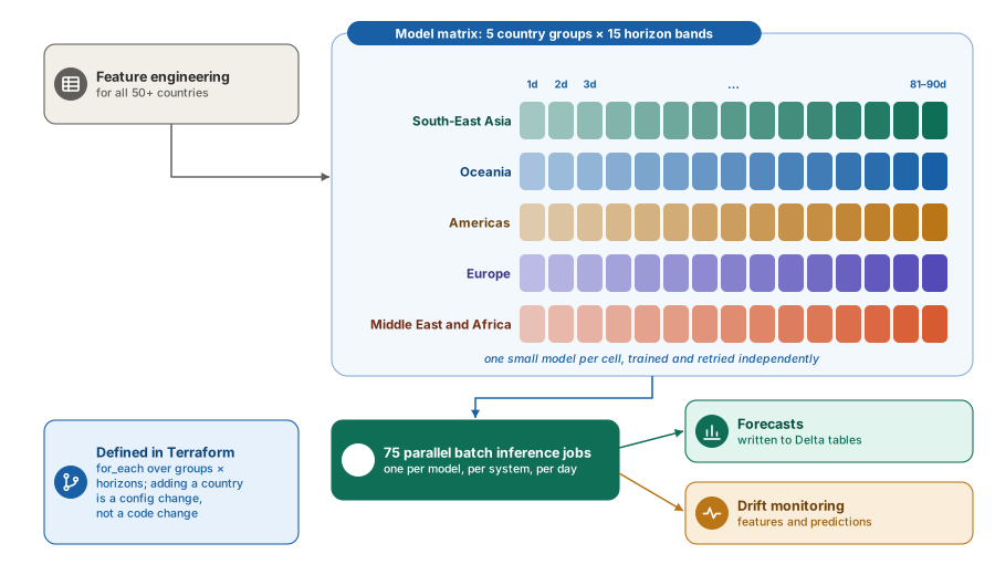
Country groups are declared in Terraform, and jobs are generated with a for_each over every group and horizon combination, with deterministic model names built from the group’s country codes and horizon range. Adding a country is a configuration change, not a code change. The old launch-country models stay in the registry for rollback.
Part 1: property forecasting, the hard road
Where it broke
The original launch countries had one thing in common: years of booking history behind almost every hotel. That was quietly load-bearing.
At 50+ countries, many hotels had been onboarded in the last few months. A hotel in a launch country with six years and hundreds of stays has a clear booking pattern; a hotel in Bolivia onboarded six months ago has a handful of stays. For the second kind, every feature computed from the hotel’s own past went noisy or came back empty.
The model didn’t get worse. The data underneath it got thinner, and the features that mattered most stopped describing very much.
We tried reaching for the model first: more trees, more tuning. It moved almost nothing, which was the first useful signal. If tuning can’t recover the loss, the loss isn’t in the model.
So we went the other way and looked at the hotels the model was getting most wrong. A pattern showed up quickly: many were in last-minute markets. Guests booked days, sometimes a week, before arrival, and nothing in the feature set described that. The model saw a hotel sitting nearly empty three weeks out and read it as weak demand, when that was completely normal for how the hotel fills.
What we changed
Three changes, in this order:
- Feature engineering: give the model a signal it had never had
- Hold-out training: make our own numbers trustworthy
- A defensive data-quality fix: close a gap in the history we read
None of them was a modelling change.
1. The missing features: lead time
The model had rooms on the books, calendar position and rolling recent demand. Nothing told it how far in advance a hotel’s guests tend to book.
That matters enormously. Two hotels with identical occupancy today are in completely different positions if one fills up six weeks out and the other fills up in the last three days. Without a lead-time signal, the model can’t tell them apart, and at 90-day horizons that distinction is most of the problem.
So we derived three features per hotel from its booking curve: the cumulative room nights on the books h days before each stay.
| Feature | What it captures |
|---|---|
avg_lead_time | Booking-weighted mean of days ahead: the centre of the pattern |
lead_time_q50 | The furthest-out day by which half the eventual rooms were booked |
lead_time_q90 | The furthest-out day by which 90% were booked |
The mean gives the centre. The two quantiles give the shape: whether a hotel fills steadily or all at once. Each feature is computed per past stay, then averaged across all of the hotel’s completed stays in the 365 days before the forecast date.
Building the version we didn’t ship
Our first attempt was to be more precise: compute lead time per season and day type (month ±1, weekday versus weekend), since a beach resort clearly books differently in August than in January. The intuition was sound.
We built it end to end, trained on it and compared. It lost.
Slicing a hotel’s year into 24 seasonal cells left most cells with one or two stays, so the “precise” feature was mostly noise, and for new markets it almost always fell back to a global value. The plain yearly average won on error, and we shipped that.
I’m glad we built the losing version. “We tried it and it measured worse” is a far stronger position than “we reasoned it wouldn’t work”.
Never return null, but always record why
Even with a full year pooled, many hotels didn’t clear the minimum bar of five eligible stays. Rather than emit nulls, we borrowed from the closest comparable group:
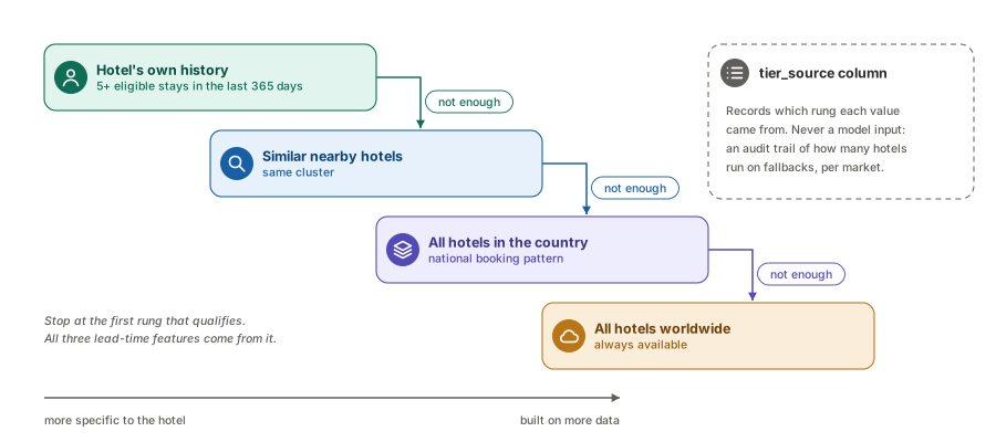
Each rung is less specific to the hotel but built on more data. You stop at the first one that qualifies, so every hotel gets a value and no nulls reach the model. All three features always come from the same rung.
The detail I’d carry to any project: we recorded which rung each value came from in a separate tier_source column. It’s never a training input. It’s an audit trail. It let us ask, at any point, how many hotels were running on their own history versus a borrowed country or global average. That’s a direct measure of where coverage is genuinely thin, and monitoring its distribution per market gives early warning of data-quality problems. That one column answered more questions than any dashboard we built.
Settle the definition before writing the query
One wrinkle cost real time. Bookings get cancelled, and sometimes rebooked. So “how far ahead do guests book?” has more than one defensible answer.
- Option A: count every booking event, including ones later cancelled
- Option B: count only bookings that stuck
We tried A first. In cancellation-heavy markets, the dip-and-recover pattern made hotels look like they booked further ahead than they did, and sometimes rooms on the books exceeded the final total, breaking the quantile thresholds. In the low-cancellation launch countries this barely showed up; at 50+ countries it distorted whole markets.
We shipped B. Using only positive booking increments, the calculation stays stable whatever a market’s cancellation rate. If is the net change in rooms booked at lead time :
The quantiles come from the cumulative positive bookings: is the largest at which half of all positive bookings were already in.
The lesson isn’t which option is correct. It’s that this was a definition problem dressed up as an implementation problem. It needed settling explicitly, and agreeing with the people who use the forecast, before anyone started building.
Every feature is also anchored to an as_of_date and uses only stays before it, so no future data leaks into training.
2. Making our own numbers trustworthy
With features changing this much, we needed to be certain that an improvement was real and not an artefact of how we scored ourselves. So we split training into two phases:
- Hold-out search: train on earlier data only, and tune and select on the last three months or so, which the model never trains on. Whatever wins there wins on evidence.
- Full retrain: retrain the winning setup on all the data for production, but keep reporting the hold-out score, not a re-score after the retrain.
Re-scoring after the full retrain always looks better, because the model has now seen that data. That number is optimistic by construction, and quoting it is how teams get surprised in production.
This changed no predictions, but without it we’d have been tuning against a flattering mirror.
3. A defensive fix on the history we read
The warehouse tracks hotel records as a slowly changing dimension (SCD type 2). When a hotel updates its name or address, it gets a new record key, and booking snapshots captured before the update stay under the old key. Our feature pipeline grouped by hotel, record key and stay date, so a hotel that changed its details mid-curve was read as two half-empty booking curves instead of one complete one. That produced wrong lead-time values.
The fix was one line: drop the record key from the grouping, so every version of the hotel folds back into a single curve.
# Before: the record key splits one booking curve into partial rows
pivoted = df.groupBy("hotel_id", "record_key", "stay_date").pivot("lead_days")

# After: all versions of the hotel merge into one complete curve
pivoted = df.groupBy("hotel_id", "stay_date").pivot("lead_days")
Upstream reconciliation caught most cases, so this was intermittent, but the shape is worth noting. In the launch countries, with their deep history, hotels rarely changed their details and there was history to spare. Newly onboarded hotels update their details constantly, and they’re exactly the ones with no history to lose. Scale didn’t introduce the bug. It removed the cushion that made it harmless.
Caught in a cutover rehearsal
One more issue surfaced in preprod, during a cutover rehearsal. When we retired an old country group, one of the original countries briefly belonged to both the old and new groups. Drift monitoring filtered predictions by country code only, picked up leftover rows from the retired model, and crashed looking up a training score that routine MLflow cleanup had already deleted. Because a prediction for horizon h is made h days ahead, each horizon stayed broken for exactly h − 1 days. The fix was to filter by model name too, since it already encodes the country group and horizon, so old rows are excluded on every future cutover.
Part 2: market forecasting, the fast road
Why MDF scaled fast
MDF forecasts demand for a whole geographic cluster of hotels, then splits it across properties by fair-share ratios. A cluster has hundreds of stays where a single new hotel might have five. Aggregation is a natural cure for sparsity. The market-level signal didn’t thin out the way one hotel’s history did, so the core pipeline needed no redesign. Only the scope of the data grew.
MDF’s own wrinkle: clusters don’t respect borders
Geo-clusters group hotels by proximity and market behaviour, not by country. A cluster on a land border can legitimately contain hotels from two countries. With only a few launch countries in scope, none of them neighbours, this never came up. Across Europe and the Americas, cross-border clusters are common. So who trains on that cluster, and who writes its predictions?
Separately, inference upserted predictions into a shared Delta table with MERGE, and 75 concurrent jobs caused occasional conflicts.
One rule fixed both
Whoever has the most properties owns the cluster. A new first task in feature engineering counts active properties per country in each cluster and assigns the cluster to the country with the most, breaking ties alphabetically so the result is deterministic. Clusters dominated by countries outside the target list are excluded.
That single lookup table, computed once per run and shared by all 150 training and inference jobs, did two things:
- Scoped training: each country group trains only on the clusters it owns
- Made writes disjoint: each inference job writes predictions only for properties in its own clusters, so no two jobs ever write the same property and the
MERGEsucceeds without conflicts at any level of concurrency
That one table is what let MDF’s scale-up ship in two weeks instead of needing a rebuild.
The results
| Before | After | |
|---|---|---|
| Countries covered | a few | 50+ |
| Country groups | 1 | 5 |
| Training / inference jobs per system | 15 / 15 | 75 / 75 |
| Properties receiving MDF forecasts | a few thousand | tens of thousands |
| MDF geo-clusters | ~150 | 500+ |
Delta MERGE conflicts | occasional under load | zero |
For accuracy, here’s the test NMAE (lower is better) for each new country group compared with the original launch-country model, at short, medium and long horizons. These are approximate values read from our evaluation charts:
Property forecasting (PDF)
| Model | 1 day | 15–21 days | 81–90 days |
|---|---|---|---|
| Original launch countries | ~0.07 | ~0.24 | ~0.38 |
| South-East Asia | ~0.08 | ~0.25 | ~0.36 |
| Oceania | ~0.07 | ~0.23 | ~0.34 |
| Americas | ~0.08 | ~0.25 | ~0.38 |
| Europe | ~0.06 | ~0.20 | ~0.34 |
| Middle East and Africa | ~0.08 | ~0.23 | ~0.27 |
Market forecasting (MDF)
| Model | 1 day | 15–21 days | 81–90 days |
|---|---|---|---|
| Original launch countries | ~0.035 | ~0.08 | ~0.15 |
| South-East Asia | ~0.03 | ~0.08 | ~0.15 |
| Oceania | ~0.02 | ~0.06 | ~0.11 |
| Americas | ~0.04 | ~0.10 | ~0.17 |
| Europe | ~0.035 | ~0.08 | ~0.13 |
| Middle East and Africa | ~0.03 | ~0.13 | ~0.19 |
For PDF, with lead-time features in place, every new group now matches or beats the original launch-country error at long horizons, and Europe beats it at every horizon, while covering far more of the world with an essentially unchanged model architecture. The lead-time features did the overwhelming majority of that work. The Middle East and Africa group covers few hotels, so its numbers are the least reliable.
MDF tells a more mixed story: Oceania and Europe come in below the original model, South-East Asia matches it, and the Americas and Middle East and Africa groups are higher, especially at longer horizons. Those are the obvious places to look next.
What I’d take to the next project
- The biggest accuracy win came from a feature, not a model. Lead-time features moved the numbers more than any amount of tuning. When accuracy drops, the instinct is to reach for the model. More often, the leverage is in giving the model a better view of the problem.
- If tuning can’t recover a regression, the regression isn’t in the model. A cheap, fast diagnostic.
- Design for the entities with no history. A feature computed from one hotel’s past is only as good as that past. Deciding up front what happens when it’s thin, with a fallback that always returns something and records where it came from, is most of the work.
- Make a refinement prove it earns its complexity. Seasonal lead time was the more sophisticated feature, and it measured worse. Building it and comparing gave us an answer. Reasoning about it would only have given us an opinion.
- Fix your evaluation before you trust your improvements. Every gain above was believable only because we had an honest hold-out window to measure it on.
- Scaling ML is a data-quality problem before it’s a modelling problem. The hard bugs were about what the data meant, not the model.
- Aggregate features scale more gracefully than entity-level features. MDF scaled in two weeks; PDF took over a month. That’s worth knowing before you commit to a feature’s granularity.
- Config-driven, independent stages make scaling cheap once the data is right. Adding a country became a Terraform variable. For PDF we added one pipeline stage and modified two; the rest were never touched.
What’s next
The weaker MDF groups show where accuracy needs work next, and the fallback audit column, monitored per market, shows where coverage is still thin.
The takeaway
Same model, more of the world, and accuracy fell off a cliff. We got it back, and for property forecasting beat the original in most groups, by giving the model a signal it had never had, measuring ourselves honestly and fixing what the data actually meant. The model was never the problem.
If you’re scaling forecasting or other ML systems across markets, I’d love to compare notes. Find me on LinkedIn.