Recommender systems are among the most widely used data science capabilities in industry, and among the hardest to evaluate correctly. A popularity baseline costs almost nothing to build and often lands within a small factor of far more elaborate models. Showing that a new model really beats it, and that the gain belongs to the model rather than to the evaluation setup, turns out to be harder than building the models.
So I built the whole stack and then spent as long again trying to break my own results. Five parts:
- Classical baselines at real scale — popularity, item-item CF, ALS and BPR on 15.6M interactions, behind one unit-tested evaluation harness.
- The production two-stage architecture — FAISS retrieval into a LightGBM reranker, measured for accuracy and for where the milliseconds go.
- Personalisation beyond one accuracy number — cold start, customer segments and popularity bias on real retail data.
- Whether deep learning pays for itself — a two-tower model trained on GPU, plus three published neural architectures on identical data.
- External validation — the same algorithms re-run through an independent framework, and against published numbers under a matched setup.
Part V is the part that usually gets skipped, and it was the most useful. It turned up a bug in the popularity baseline that an established open-source framework has been measuring against for years, and two under-tuned configurations in my own code. Neither produced an error message.
One finding runs through all five: a reported accuracy figure can’t be interpreted without the evaluation protocol that produced it. Changing only what the held-out item is ranked against moved Recall@10 by a factor of 7 to 12 on identical data, and reversed the ranking of two settings of the same algorithm.
Everything below is reproducible. The code, the configs and the result logs are on GitHub (linked at the end of this post), and the logs are committed deliberately, so every number here traces back to the row that produced it.
| Datasets | MovieLens 25M (15.6M interactions, 162K users, 24K items), MovieLens 1M, H&M Personalized Fashion (3.7M purchases, 379K customers) |
| Built | Evaluation harness, 4 classical baselines, FAISS + LightGBM two-stage pipeline, two-tower neural retriever, cold-start routing layer |
| Stack | Python, implicit, FAISS, LightGBM, PyTorch, Polars, RecBole, uv |
| Measured | Recall@10, NDCG@10, MRR, coverage, novelty, intra-list similarity, popularity bias, per-request latency |
Part I: classical baselines, done carefully
I started with MovieLens 25M: 25 million ratings, large enough that implementation choices have consequences, with real timestamps and the densest body of published results of any public dataset.
Two quiet decisions shaped everything after:
- Explicit to implicit. All the models here are implicit-feedback methods, so I kept ratings of 3.5 stars and above as positives. A 1-star rating is evidence of dislike, not a weak “like”.
- Iterative 5-core filtering. Removing low-activity users can push items below the threshold and vice versa, so the filter loops until nothing changes. That left 15.6 million interactions, 161,572 users and 23,965 items. Most of the reduction came from the core filter, not the rating threshold.
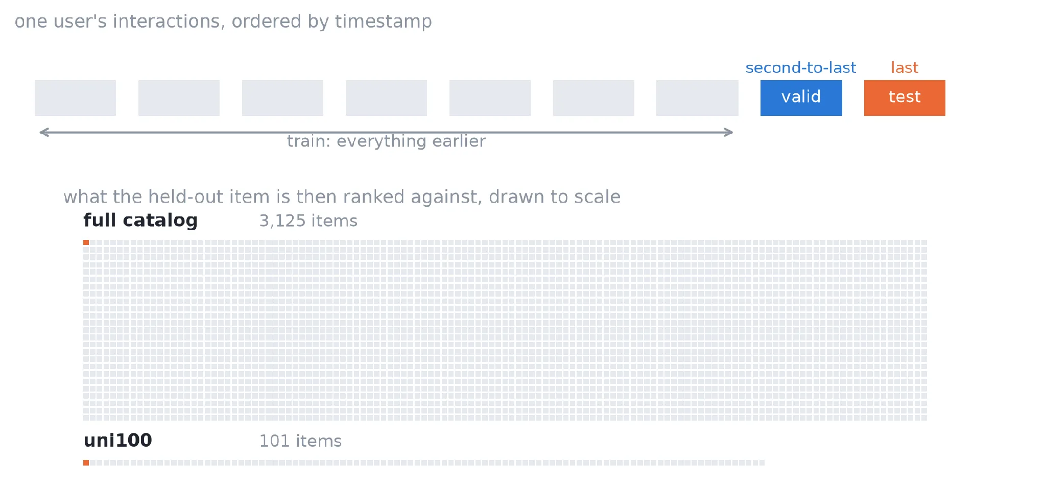
The split was leave-one-out by time: each user’s latest interaction is the test item, the one before is validation, and everything earlier is training, with an assertion that nothing leaks backwards.
The less visible deliverable mattered more than the models: one evaluation harness, unit-tested against hand-computed cases and then left alone, that every later result runs through. It ranks the held-out item against the full catalog, not a sample, which is stricter than much of the literature (Part V shows by how much). Alongside accuracy, it tracks coverage, novelty, intra-list similarity and popularity bias.
| Model | Recall@10 | NDCG@10 | Coverage@10 | Novelty@10 |
|---|---|---|---|---|
| Popularity | 0.0491 | 0.0247 | 0.008 | 8.23 |
| Item-item CF | 0.0797 | 0.0414 | 0.096 | 8.98 |
| BPR | 0.0812 | 0.0403 | 0.530 | 12.36 |
| ALS (α = 20) | 0.0966 | 0.0470 | 0.156 | 9.93 |
| ALS (α = 1) | 0.1044 | 0.0534 | 0.056 | 9.62 |
Three things stood out:
- Every personalised model beats popularity, but only by about 2×, against a baseline with no training and no hyperparameters.
- One hyperparameter mattered more than the choice of algorithm. Moving ALS’s confidence weight α from 20 to 1 improved NDCG@10 by 14%, more than the whole gap between item-item CF and BPR.
- Accuracy and coverage pull in different directions. The most accurate model recommends from 6% of the catalog; BPR is third on accuracy but first on coverage and novelty. That’s a product decision, not a modelling one.
And a Recall@10 of 0.10 doesn’t mean the system is wrong 90% of the time. It has to place one specific item in a top 10 out of nearly 24,000. Random guessing scores 0.04%, so the best model is about 250 times better than chance.
Part II: two-stage retrieval and ranking
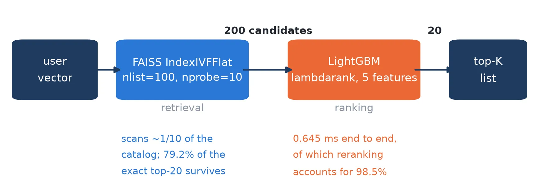
Production systems don’t score the whole catalog for every user. They retrieve a few hundred candidates cheaply, then rerank those with a richer model. I built that: FAISS (an inverted-file index over ALS item embeddings, searching a tenth of the catalog) retrieving 200 candidates, and a LightGBM lambdarank reranker over features such as the retrieval score, item popularity, user activity, the item-item CF score and genre affinity.
The first version scored below popularity. For 62% of training queries, the held-out item wasn’t among the retrieved candidates, so the pipeline injected it to create a positive example. Injected rows necessarily had poor retrieval scores, since good ones would have been retrieved, and because they were the majority, the reranker learned that its most informative feature was uninformative. One binary is_injected feature let the model separate the two cases. Recall@10 rose 93%. In production nothing is injected, so the flag is always zero.
Even fixed, the two-stage pipeline reached only about 84% of its own ALS base model’s accuracy. That lines up with the measured ceiling: only 79% of the items exact scoring would choose survived approximate retrieval. The reranker can only order what retrieval hands it. What it did buy was diversity: three times the catalog coverage.
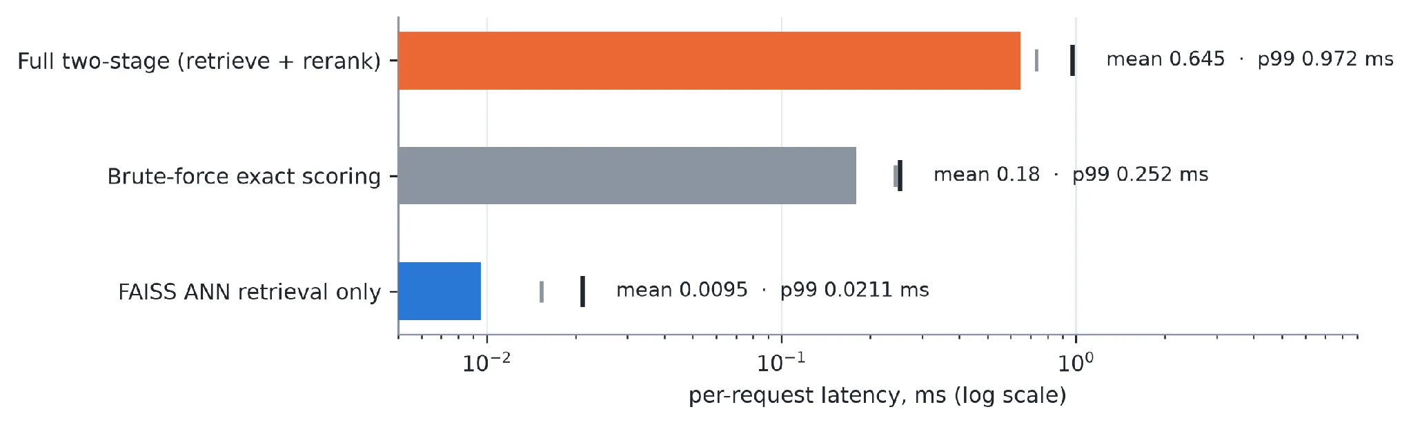
The most transferable lesson: the accuracy and latency bottlenecks were in different stages. Accuracy was limited by retrieval; latency was dominated by reranking, about 98.5% of a 0.645 ms request. At this catalog size, exact scoring was actually faster than the whole pipeline. FAISS’s 19× speed-up matters at larger catalogs; here, measuring it established the method and the accuracy cost.
Part III: cold start, segments and popularity bias
One averaged accuracy number can’t tell you what happens to a customer you’ve never seen, whether quality is spread evenly, or how much of a “personalised” list is just bestsellers. Those questions need real customer attributes and timestamps, so I moved to the H&M Personalized Fashion dataset: a 90-day window with 379,000 customers, 28,000 articles and 3.7 million purchases. It’s about ten times sparser than MovieLens, with roughly 8 interactions per customer against 94.
The model ranking reversed
With unchanged hyperparameters, two findings from MovieLens flipped:
| Model | MovieLens 25M | H&M |
|---|---|---|
| Popularity | 0.0491 | 0.0093 |
| Item-item CF | 0.0797 | 0.0958 |
| ALS (best α) | 0.1044 (α = 1) | 0.0843 (α = 20) |
| BPR | 0.0812 | 0.0455 |
- Item-item CF overtook matrix factorisation. ALS has to estimate a 64-dimensional vector per customer from about 8 observations. Item-item CF estimates nothing per user; it needs item co-occurrence, and with hundreds of thousands of customers the item side stays dense even when the user side doesn’t.
- The best α inverted. On a much sparser matrix, the few positives have to be weighted heavily or they’re drowned out. A hyperparameter inherited from a paper, or from a previous project, is a guess.
One average hides a lot
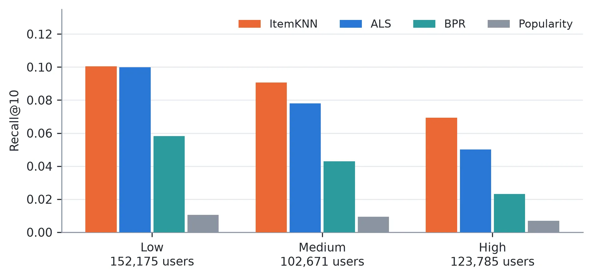
- More active customers were harder to predict, for every model. Low-activity customers tend to rebuy a narrow set of basics, which predicts one step ahead well. Busy customers shop across many categories.
- Age barely mattered (about an 11% spread), but membership status did: customers still at the pre-registration stage scored Recall@10 of 0.153 against active club members’ 0.087, a 76% lift, with the same ordering for every model.
- Item-item CF’s win was uniform, holding in every activity tercile and age band, not just on average.
Cold start fails silently
Leave-one-out can never produce a genuinely new customer, since every test user appears in training. A global 14-day time split can: 10,501 of 62,306 evaluated customers had no history at all.
| Model | Warm customers | Cold customers |
|---|---|---|
| Popularity | 0.0084 | 0.0119 |
| Item-item CF | 0.0174 | 0.0002 |
| ALS (α = 20) | 0.0190 | 0.0002 |
| BPR | 0.0085 | 0.0000 |
This isn’t graceful degradation. It’s a mechanical failure. With no interactions, ALS solves to a zero user vector, and item-item CF multiplies a zero row by the similarity matrix. Both score every item zero, fall through to the same index-order tie-break, and hand every new customer an identical fixed list of ten items unrelated to anything. Their cold-start recall was bit-for-bit identical. No error, no warning.
Popularity was the only one of the four that produced a meaningful ranking for new customers, and it actually did better for them than for existing customers, perhaps because a first purchase skews towards what’s trending.
So I added a routing wrapper that sends customers with no history to a fallback, and compared three: plain popularity, popularity by age band, and recency-weighted popularity (a 7-day half-life, effectively “trending now”). Age-band popularity was best for the single top slots; recency pulled clearly ahead by K = 20 (+85% over plain popularity). Across all customers, the fallback lifted Recall@10 by 15–33%. A cheap fix, but only if you know to build it.
How much is just bestsellers?
A direct popularity-bias metric (the share of recommendations drawn from the top 1% of items) showed item-item CF’s win was real personalisation: 9% of its slots were bestsellers, against 44% for ALS, which was also less accurate.
On H&M, the two-stage pipeline won outright: 17% better Recall@10 than item-item CF, the opposite of MovieLens. Approximate retrieval kept 91% of the exact candidates, and the reranker had genuinely complementary signal, including the item-item CF score from the dataset’s strongest single model. Model rankings are a property of the data, not the algorithm.
Part IV: does deep learning justify its cost?
I tested that two ways.
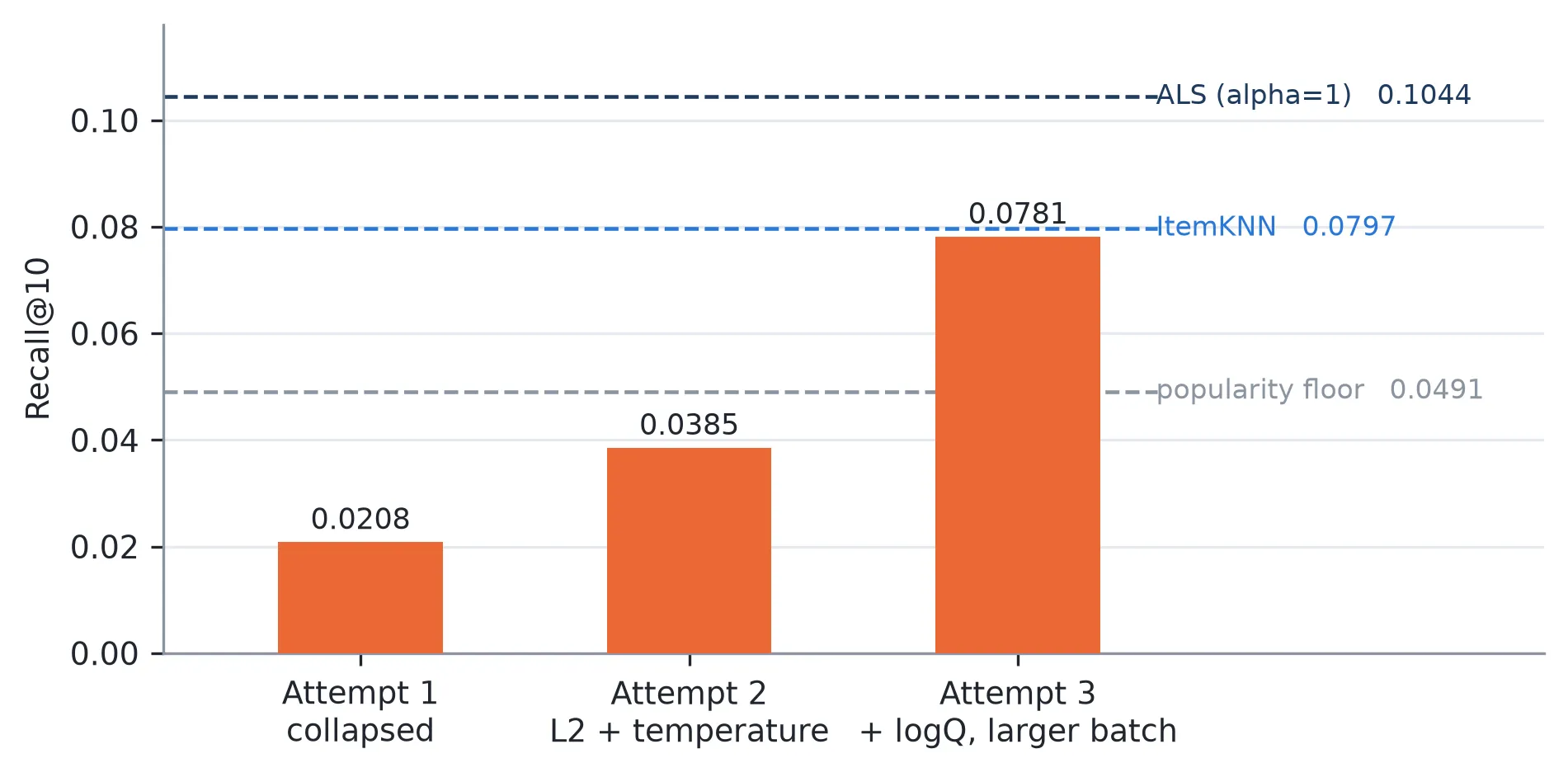
A two-tower model I built from scratch, matched to ALS’s 64 dimensions and trained on GPU with in-batch sampled softmax, then evaluated through the same harness. It took three attempts:
- Collapse. It scored below popularity. Intra-list similarity of 0.9997 gave it away before any retraining: every recommended item looked the same. The network had learned item magnitude instead of direction. L2-normalising both towers plus a temperature of 0.05 fixed the collapse.
- Still below popularity. Popular items were being unfairly penalised as in-batch negatives. A logQ correction, larger batches and more epochs addressed that.
- Parity, within 2–4% of item-item CF and BPR, but still well short of ALS.
Three published neural models (NeuMF, LightGCN and Mult-VAE), trained by the RecBole framework on identical MovieLens 1M data: Mult-VAE tied item-item CF, and NeuMF and LightGCN finished below both item-item CF and BPR.
Both lines of evidence point the same way, and they arrive at the best-known result in the reproducibility literature from my own data rather than by citing it: well-tuned classical methods are a very hard bar. ALS got its result in minutes on a laptop CPU. Matching weaker classical models with a neural one took a GPU, a training pipeline and debugging two failure modes, neither of which produces an error message. The failures were only diagnosable because I tracked intra-list similarity, novelty and coverage alongside accuracy from the start.
The caveat matters: both datasets are identifier-only, with no item text, images or rich context. That’s where neural models have the least room to shine, so this isn’t evidence that deep learning doesn’t help recommendation in general.
Part V: external validation
Parts I–IV hold everything fixed, so they rank models against each other. They say nothing about where those models stand relative to anyone else’s work. Part V tested that three ways.
An independent implementation
I ran RecBole on exactly the same folds. Its “benchmark file” setting bypasses its own filtering and splitting, so both systems hold out identical items for identical users. Before that, I let both preprocess the raw data independently: they converged on identical users, items and interactions, ruling out preprocessing as an explanation for later differences.
One near-miss is worth sharing. RecBole selects the best epoch on the validation fold, then reports on it. On validation, Mult-VAE, NeuMF and BPR all appeared to beat item-item CF. On the test fold, item-item CF was first. Had I compared validation to validation, as originally planned, this post would have said neural models won.
The protocol changes the ranking, not just the score
Then I changed only the candidate set: the full catalog versus 100 sampled negatives, the protocol popularised by the NCF paper and widely used on MovieLens since.
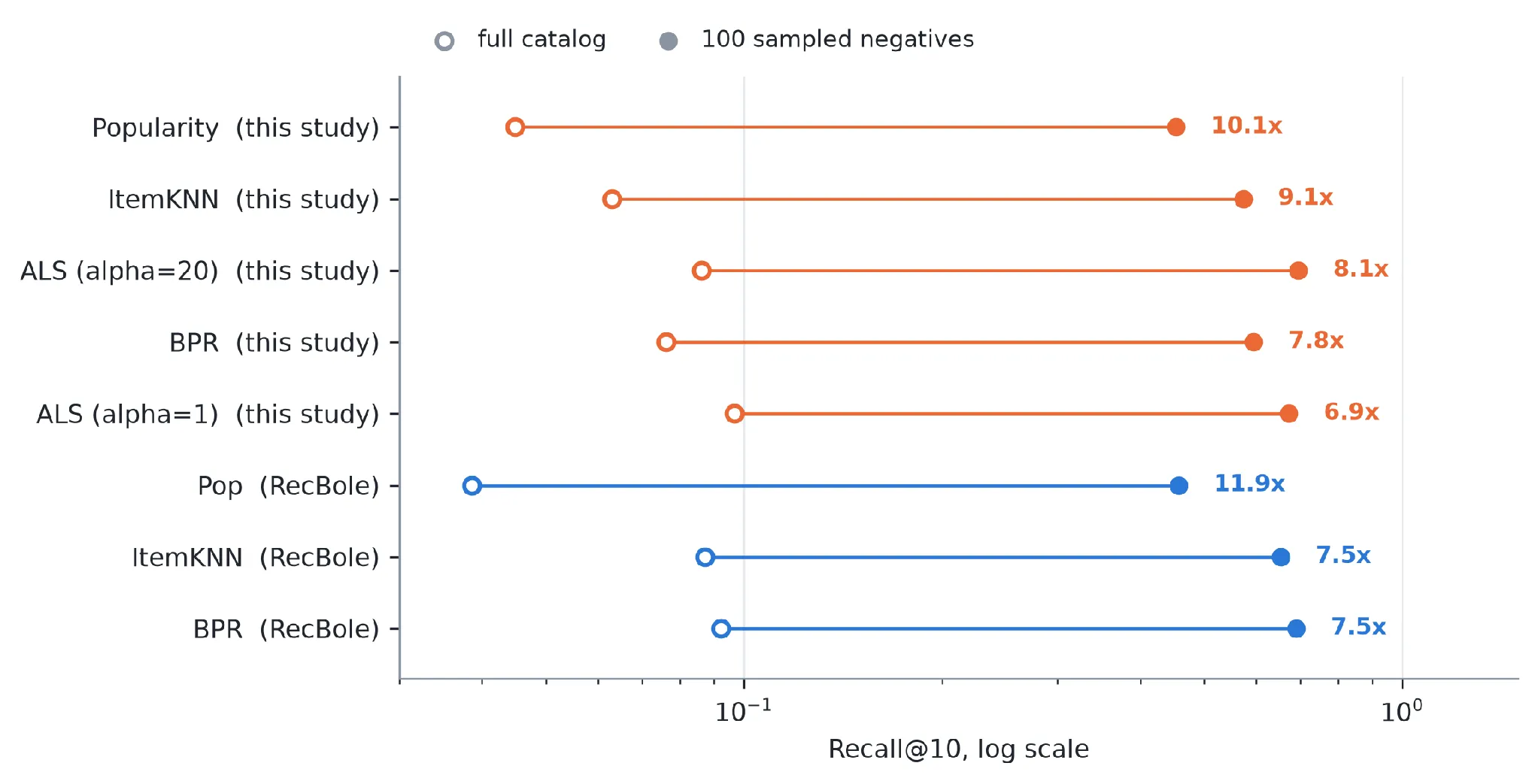
- Accuracy moved by 7–12×, on two independent codebases. For comparison, the entire spread from the popularity floor to the best model is about 2×.
- The ranking changed. Under full-catalog ranking ALS with α = 1 beat α = 20; under sampled negatives it reversed. If a protocol can reorder two settings of the same algorithm, a sampled-negative leaderboard is unreliable even for relative claims.
- Popularity is inflated most (10–12×), so the common protocol understates how much personalised models beat the baseline.
A bug in the baseline everyone is measured against
Popularity was my control: the same trivial algorithm in both codebases should agree. It didn’t, and tightening the setup made the gap worse. Ruling out the obvious explanations one by one led to RecBole’s learned item counts: every one of its top 20 items had a count of exactly 275, against true counts from about 1,700 to 2,800.
The cause was one line. RecBole’s popularity model increments counts with a PyTorch indexed assignment over a batch of item IDs. With duplicate indices, that credits an item +1 per batch, not +1 per interaction, so counts saturate for anything popular and the head of the ranking is destroyed. Replacing it with torch.bincount brought the two systems into agreement to four decimal places.
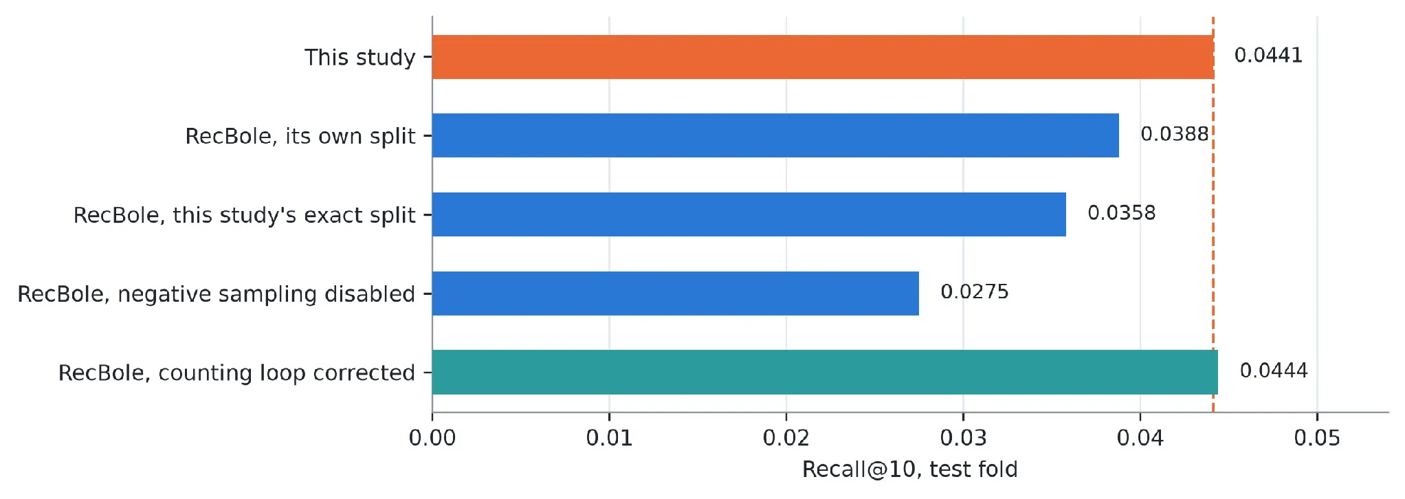
That baseline was understated by 14–22%, by an amount that varies with batch size and epochs. Every margin measured against it is inflated by a different amount per experiment. It only showed up because an independent implementation of a trivial algorithm existed to disagree with it.
Matching published numbers
Finally, I reproduced the NCF paper’s exact setup: every rating a positive, no core filtering, 100 sampled negatives. My ALS landed inside the paper’s reported range for its closest relative (eALS), and within 3% on HR@10 of NeuMF without pre-training. Since the original NCF code reportedly picked epochs on the test set, matching it closely is a stronger result than it looks.
And where my own code fell short
The comparison cut both ways. It showed my BPR was under-trained (a fixed iteration budget that didn’t scale with data) and my item-item CF configured differently (200 neighbours, no shrinkage). Two unrelated references, RecBole and the NCF paper, pointed at the same two models in the same direction.
Lessons learned
- Record the protocol with every number. Dataset version, preprocessing, split and candidate set all have to match before two numbers can be compared. The candidate set alone moved results 7–12× and reordered models.
- Build a well-tuned classical baseline first. Popularity, item-item CF and ALS set a bar that took a neural model three attempts to reach.
- Model rankings don’t transfer between datasets. Item-item CF versus ALS, the best α, and whether two-stage helps all flipped with data density. Recommend an algorithm together with the density figures that justify it.
- Measure beyond accuracy from day one. Intra-list similarity diagnosed representation collapse, and novelty and coverage confirmed the logQ fix. A single average hid a 45% spread by activity and a total cold-start collapse.
- Build cold start deliberately. The models fail silently for new users. A routing wrapper with a trending fallback is cheap.
- Know where your bottlenecks are. In two-stage systems, accuracy was capped by retrieval and latency was spent in reranking. Optimise the stage that binds.
- Validate against an independent implementation. It found a bug in an established framework and two under-tuned models in my own code. Neither produced an error message.
What’s next
- Fix the two under-tuned configurations: early stopping for BPR, and neighbour count and shrinkage for item-item CF
- Run multiple seeds, so the threshold for a meaningful difference is measured rather than assumed (every number here is a single run)
- Add EASE, a closed-form linear model that’s consistently strong in the reproducibility literature
- Test where neural models should win: item metadata, text and images, and sequence models such as SASRec and BERT4Rec
- Build a content-based cold-start fallback that personalises from whatever is known at sign-up
The takeaway
Building a recommender is a few weeks of work. Making a claim about one that survives outside scrutiny took as long again, and it is the part that decides whether the first half was worth anything. Hold the protocol fixed, start from strong classical baselines, measure more than accuracy, and check your results against someone else’s implementation. And when someone shows you a recommender number, ask how it was measured before asking whether it’s good.
If you’re working on recommender systems, I’d love to compare notes. Find me on LinkedIn.