When a business expands into new countries, support has to be ready on day one. Someone has to decide how many agents, in which languages, for which parts of the product, and sign vendor contracts on that basis months in advance. Get it wrong one way and customers wait; get it wrong the other way and you pay for idle capacity.
This post is about how we forecast support demand for exactly that decision, for a large online advertising platform expanding into new markets. The forecasts guided the vendor capacity contracts for those markets and saved about $70K.
The catch: new markets have no history
You can’t forecast a market that hasn’t launched. So we forecast the next best thing: comparable markets, six established countries the business considered similar to the expansion markets, with the same languages and products. Their support volumes, by language and product area, were the basis for planning the new ones.
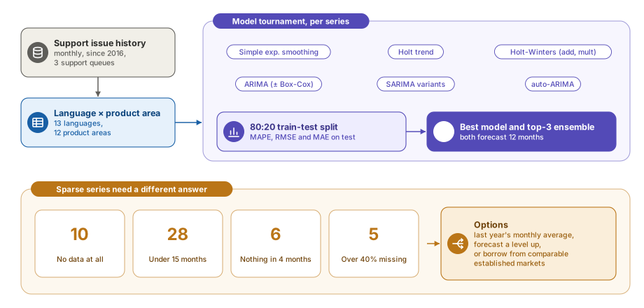
The data came from three support queues (ad quality, traffic quality and technical support), with monthly issue volumes going back to January 2016.
Choosing the right granularity
The first real decision was what to forecast. Capacity is planned by language (which agents you need) and product area (which skills they need). That gave us 13 languages × 12 product areas, about 110 series with data.
We started at country and queue level, then moved to language × product area, because that’s how capacity is actually bought. The trade-off is that finer series are sparser, and sparsity became the central problem of the project.
A model tournament for every series
There was no reason to believe one model would suit every language and product area, so each series ran its own tournament:
- 14 model configurations: simple exponential smoothing, Holt’s trend method, additive and multiplicative Holt-Winters, ARIMA with and without a Box-Cox transform, four seasonal ARIMA (SARIMA) variants and three auto-ARIMA variants.
- An 80:20 time-based split, training on the earlier months and testing on the most recent.
- Three error measures on the test set: MAPE, RMSE and MAE. MAPE is easy to explain to the business, but it explodes on small volumes, so RMSE and MAE kept us honest on low-volume series.
- Two forecasts per series for the next 12 months: one from the single best model, and one from an ensemble of the top three. Negative forecasts were capped at zero.
Across the 60 series with enough history to model, the results justified the tournament:
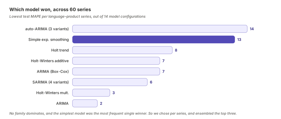
No family dominated. Simple exponential smoothing, the simplest model in the set, was the single configuration that won most often. Seasonal models won less often than you might expect, most likely because many series were too short or too noisy for seasonality to be estimated reliably.
Accuracy varied a lot by series. Large, stable series forecast well; thin ones didn’t. We generally planned with the top-3 ensemble, because it’s less sensitive to one model getting lucky on the test window.
Sparse series need a different answer
Around 50 language × product-area combinations had too little data to model at all. We wrote the criteria down so it wasn’t a judgement call each time:
- No data at all: 10 combinations
- Fewer than 15 months of history: 28
- Nothing in the last 4 months: 6
- More than 40% of months missing between the first and last observation: 5
For these, a model would only produce confident-looking noise. Typically these were a niche product area in a smaller language, with zero to 14 issues in the past year. The options we put to the business were deliberately simple:
- Use last year’s monthly average as the forecast.
- Forecast one level up (the product area across languages) and allocate down.
- Borrow from comparable markets where the same combination was better established.
For capacity planning, a simple, defensible number beat a sophisticated wrong one.
The pandemic year
The data included March 2020 to February 2021, when support patterns changed sharply. Training on it risked teaching models a pattern that wasn’t coming back; dropping it threw away a year of an already short history.
We ran both: one set of models trained on all the data, and another that excluded the pandemic year, then compared and combined the forecasts. Later, we compared both against actual volumes as they came in, to see which version was tracking reality.
Lessons learned
- Forecast at the level decisions are made. Language × product area was harder than country totals, but it’s what capacity contracts are written in.
- Let each series choose its model. With 14 configurations and no consistent winner, a per-series tournament with a top-3 ensemble beat any single global choice.
- Write the sparsity rules down. Explicit criteria for when not to model saved endless debate and stopped noise from looking like a forecast.
- Use more than one error measure. MAPE alone punishes low-volume series unfairly; RMSE and MAE balanced it.
- Treat shocks as a modelling choice. With and without the pandemic year were both defensible; running both and checking against actuals was better than guessing.
- Simple models are strong baselines. Simple exponential smoothing winning most often is a useful reminder to always include the simplest model.
The takeaway
Forecasting for markets with almost no history is mostly about deciding what you can honestly forecast, and being explicit about what you can’t. A per-series tournament, ensembles for stability, written rules for sparse data and a clear view on the pandemic year gave the business numbers it could sign contracts on, and saved real money in the process.
If you’re forecasting demand with thin data, I’d love to compare notes. Find me on LinkedIn.